Abstract
Artificial intelligence is transforming labor markets around the world, yet we do not completely understand its effects on individuals. Previous research has used aggregated data and proxies, which fails to isolate the impact of AI on different tiers of the workforce. We therefore investigated whether AI penetration in firms has a causal effect on the displacement of routine labor and the complementarity of creative and complex work.
Our dataset includes over 100 million job postings from 2015 to 2024. Using it, we developed a knowledge distillation system that trains an efficient student model on accurate LLM outputs as the teacher. The results were validated against 9,500 human labels. Each posting was categorized as routine, complex or creative and given an intensity score, producing a panel across 72 countries.
A one-unit increase in AI intensity reduced routine labor demand by 2.1 percentage points and increased creative labor demand by 1.8 percentage points. The effects strengthened over three years after adoption and were twice as large in higher-income countries. To establish causality we used event-study and instrumental-variable designs. We also built a forecasting system using semantic embedding features and a temporal deep learning model, which reduced prediction error by 18–31% against established baselines. We conclude that AI adoption is driving a structural reallocation of labor demand: it substitutes for routine labor and complements complex and creative labor.
Keywords — Large Language Models; Computational Social Science; Labor Market Dynamics; Time-Series Forecasting; Natural Language Processing.
1Introduction
In recent years, artificial intelligence — machine learning, large language models, automation technologies — has penetrated economic and social sectors at an unprecedented pace. The process is inherently double-edged: AI substitutes for repetitive labor while spawning new occupations such as prompt engineers and AI ethicists. This duality has ignited an ongoing debate between policymakers, industry leaders and scholars, and yet our understanding of AI's current impact on the labor market remains surprisingly unclear, fluctuating between optimistic predictions and dystopian anxieties.
Significant gaps persist. Much of the literature focuses on macro-level effects such as industry-level employment substitution rates, or on single mechanisms — a substitution effect, or a creation effect, but rarely both at once. AI application is often measured with superficial methods such as keyword searches for “AI” or “machine learning”, which fail to capture the actual depth of AI penetration in enterprises. Coupled with unresolved endogeneity — high-skill enterprises may proactively adopt AI and adjust labor structures — these limitations undermine the reliability of causal inference.
To address these gaps we employ a large-scale dataset of over 100 million online job postings gathered from major international recruitment sites between 2015 and 2024. We construct a novel indicator, AI Intensity for Employment (AIFE), which quantifies the extent to which specific occupations are susceptible to transformation driven by AI integration. Because web-scraped data is unstructured and high-dimensional, we employ a three-stage knowledge-distillation pipeline consisting of entity resolution, teacher–student distillation with human-in-the-loop calibration, and systematic evaluation against established baselines.
We then apply econometric methods to establish causality and alleviate endogeneity. We construct a Two-Way Fixed Effects model to isolate the effect of changes in AIFE on labor composition, verify the parallel-trends assumption with a dynamic event-study design that addresses heterogeneous treatment effects across cohorts, and alleviate remaining endogeneity concerns with a Bartik-style shift-share instrumental variable. Finally, in response to the absence of forward-looking frameworks, we develop a predictive pipeline that introduces Semantic Leading Indicators — high-dimensional features derived from model embeddings that detect adoption momentum latent in scalar scores — integrated into a Temporal Fusion Transformer with a causal-consistency regularizer and conformal prediction intervals.
Contributions
- A scalable knowledge-distillation pipeline for economic measurement (§4). The AIFE pipeline distills the reasoning capabilities of a frontier LLM into a high-throughput encoder, processing 100 million documents at a total cost of $410. Systematic evaluation against eight baselines — keyword dictionaries, published exposure indices, GPT-4o zero-shot and fine-tuned BERT — shows the full pipeline achieves ρ = 0.931 with human consensus, a 91% improvement over keyword methods and a 16% improvement over GPT-4o zero-shot.
- Credible causal evidence at the firm level (§5). We provide firm-level causal estimates of AI adoption on hiring composition using a global dataset. Event-study dynamics with parallel-trends validation, a heterogeneity-robust difference-in-differences estimator, and a shift-share IV strategy together constitute a multi-pronged identification approach addressing the key threats to validity.
- A predictive early warning system with distribution-free uncertainty quantification (§6). Because the causal analysis quantifies the downstream consequences of AIFE increases, predicting AIFE trajectories is equivalent to predicting labor-market disruption with known effect sizes. Conformal prediction provides coverage guarantees on the resulting displacement forecasts.
2Literature Review
2.1 · Technological progress and the labor market
Early studies were grounded in the Skill-Biased Technological Change framework (Katz and Murphy, 1992; Acemoglu and Autor, 2011), which posits that technological change complements high-skilled labor while substituting for low-skilled labor, raising skill premiums and inequality. SBTC struggles to explain the job polarization observed in Europe and the United States since the 1990s, where employment grew in high- and low-skill jobs while medium-skill jobs shrank (Goos and Manning, 2007; Autor and Dorn, 2013). Routine-Biased Technological Change has since become the mainstream framework, shifting the unit of analysis from skills to tasks and emphasizing that technology substitutes for routine tasks rather than for labor of a given skill level.
2.2 · The impact of AI on labor demand
Research on mechanisms focuses on several dimensions. The displacement effect: AI reduces demand for routine labor by automating repetitive, rule-based tasks — OCR, RPA and chatbots in document processing, data entry and customer service (Frey and Osborne, 2017; Graetz and Michaels, 2018). The productivity effect: AI enhances productivity and reduces costs, potentially boosting labor demand for non-routine cognitive work through scale expansion (Brynjolfsson and McAfee, 2014; Bessen, 2019). The new task creation effect: Acemoglu and Restrepo (2018) propose an automation–new-task balance in which technology creates tasks as well as destroying them, and generative AI is giving rise to entirely new occupational fields (Eloundou et al., 2023). Finally, skill restructuring: demand for hard skills rises while the value of soft skills — communication, creativity, ethical judgement — becomes increasingly prominent (Deming, 2017).
2.3 · Generative AI
Generative AI differs from traditional AI in its labor-market impact because of breakthroughs in language understanding, content generation and complex reasoning. Zhang and Dan (2025), using Chinese recruitment data, find that hiring demand for high-exposure occupations such as accounting, editing and programming declined while demand for low-exposure occupations such as catering and nursing rose. Eloundou et al. (2023) estimate that approximately 80% of U.S. workers have at least 10% of their tasks affected by large language models, with higher exposure among high-education, high-wage occupations.
2.4 · Heterogeneous impacts
Differences across enterprises, industries and regions are central. Non-state-owned and high-tech firms are more likely to adopt AI, producing more significant labor-structure adjustments (Xu et al., 2023). Manufacturing, finance and IT services are high-frequency application sectors; face-to-face interaction-intensive service jobs such as nursing and education are less affected. Among regions, developed areas with better infrastructure and high-skilled agglomeration benefit more, whereas less-developed regions face risks of a deepening technological divide.
2.5 · Limitations of current research
Three limitations recur. First, there is a scarcity of global, high-resolution, firm-level data, as most studies rely on aggregate statistics or indirect matching. Second, AI adoption is often measured with keyword searches that fail to quantify the depth of penetration. Third, policy research tends to emphasize macro-level recommendations, lacking targeted interventions informed by micro-level mechanisms. We respond with a granular analysis of AI adoption's consequences for labor demand at the firm level, using a two-stage teacher–student framework to label hundreds of millions of postings, and accounting for regional differences in economic and technological development.
3Data Engineering
Traditional analyses of labor-market dynamics have long been constrained by the frequency and granularity of official statistics. Surveys such as the Bureau of Labor Statistics' Occupational Employment Statistics are released with significant lag and present data at an aggregate level, obscuring the high-frequency firm-level adjustments central to understanding rapid technological change.
We therefore turn to online job postings. Our data is sourced from the class-specific subsets of the Web Data Commons Schema.org extraction, built from the Common Crawl. Because our study focuses on labor demand, we use data annotated with the JobPosting type, which offers firm-level observations across numerous states and industries globally.
Web pages frequently include structured metadata in JSON-LD, Microdata or RDFa formats. WDC extracts this metadata and publishes it as N-Quads, a line-based syntax for RDF in which each statement takes the form ⟨subject, predicate, object, graph label⟩. The first three elements form an RDF triple; the fourth, the graph label, typically includes the source domain. This structure provides two advantages: transparency, since every triple can be traced back to the originating web page, and multi-graph support, so postings from many domains can be combined without losing the boundaries between their original sources.
A posting annotated with schema:JobPosting typically includes title, hiringOrganization, datePosted, jobLocation and description, plus optional fields such as employmentType, skills and qualifications. Because each posting becomes a small subgraph of many quads, we can reconstruct a rich representation of what a firm demands in terms of skills, role and location, and flag missing data when fields are absent.
The raw dataset spans January 2015 to December 2024 and consists of approximately 412 million quads — a vast but extremely noisy and heterogeneous collection. Web markup is inconsistent: the same job may be posted on multiple pages or mirrored across domains, firm names appear in many variants, and some postings omit key fields entirely. These challenges necessitate the entity resolution and deduplication steps that follow.
4The AIFE Measurement System
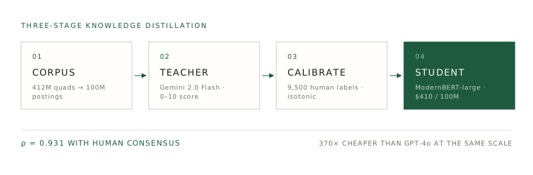
The core technical challenge is transforming over 100 million unstructured postings spanning a decade into a precise, econometrically valid firm-level panel variable. We address it with a three-stage knowledge-distillation pipeline: corpus construction and entity resolution (§4.1), teacher–student distillation with human-in-the-loop calibration (§4.2–4.4), and systematic evaluation against baselines (§4.6).
4.1 · Corpus construction
The full corpus comprises approximately 412 million RDF quads, which after deduplication on the (title, description, hiringOrganization) triple yield roughly 100 million unique postings spanning 2015–2024.
Entity canonicalization. Raw employer-name strings exhibit extreme heterogeneity — “NVIDIA”, “NVIDIA Corp.”, “NVIDIA Corporation – Santa Clara”. We employ Gemini 2.0 Flash with deterministic decoding to map each noisy string to a legally registered entity name, or UNKNOWN if no reliable mapping exists. Of 450,617 unique raw name strings observed across all years, 345,640 resolve to distinct canonical firms after aggregation, with 23.3% dropped as unknown or ambiguous. The drop rate ranges from 18.7% in North America and Western Europe to 31.2% in Sub-Saharan Africa and South Asia, reflecting both the prevalence of non-Latin scripts and lower coverage of the model's training corpus.
Sample extraction. To construct a training corpus for teacher labeling we adopt a longest-posting heuristic: for each canonical firm–year pair we retain the single posting with the highest token count. Longer postings typically contain more granular descriptions of tasks and technical requirements; selecting one posting per firm–year balances the training set at the firm level; and it guarantees each posting fits within the context window without truncation. This yields 345,640 unique postings per year — approximately N = 3,110,760 firm–year observations over the panel — which serve as the input corpus for teacher labeling. The full 100-million-posting corpus is reserved for student inference at deployment.
We acknowledge that the heuristic introduces a form of selection: it over-represents firms that produce verbose job descriptions, which tend to be larger, more professionalized employers. We quantify this bias and its effect on downstream estimates in the stratified error analysis (§4.6).
4.2 · Teacher model: zero-shot scoring
We deploy Gemini 2.0 Flash as the Teacher to produce high-fidelity soft labels for two targets: the continuous AIFE score (0–10) and a three-class task-content label (Routine, Complex, Creative). All inference uses deterministic decoding — temperature 0, top-k 1 — so that repeated calls with identical input yield identical output. Safety filters are disabled to prevent false positives on domain terminology such as “kill process” or “master/slave architecture”. The model's 1M-token context window eliminates the need for input truncation.
Prompt design. The AIFE metric must distinguish between developing AI systems and passively applying AI-embedded tools — a distinction that standard sentiment or keyword analysis cannot capture. We enforce this through a structured prompt that elicits chain-of-thought reasoning before numeric scoring, embedding three design principles: an anchored rubric of four ordinal bands with concrete exemplars, functional decomposition that instructs the model to inventory specific technical skills and distinguish using a tool from building one, and a buzzword penalty that discounts vague AI references unsupported by concrete technical requirements.
1–3 — AI-Aware / Consumer. The role uses software with embedded AI features (CRM, BI tools), but the worker does not configure or interact with the underlying model architecture.
4–7 — AI-Applied / Implementer. The role actively applies AI/ML tools to business problems. Requires understanding of model outputs, prompt engineering, or configuring pre-trained systems.
8–10 — AI-Core / Developer. The role involves researching, architecting, fine-tuning or deploying AI models. Requires deep knowledge of algorithms, loss functions and model infrastructure.
A companion prompt classifies each posting into one of three task categories. Routine tasks are repetitive, rule-based and codifiable, with success defined by adherence to a standardized process — data entry, assembly, bookkeeping. Complex tasks require high-level cognitive processing, strategic decision-making and the integration of information under uncertainty — management, engineering, surgery. Creative tasks require all the characteristics of complex work plus the generation of novel ideas, artifacts or solutions — graphic design, R&D, artistic direction.
4.3 · Student model: knowledge distillation
While the Teacher produces high-quality labels, its latency and per-token cost are prohibitive at the scale of the full corpus. We therefore distill its knowledge into a compact encoder.
Architecture. We select ModernBERT-large (395M parameters) as the Student backbone for three reasons. It supports a native sequence length of 8,192 tokens via rotary positional embeddings, which matters because 38.7% of postings exceed the 512-token limit of classical BERT, with relevant technical requirements often appearing in the tail of the document. It employs Flash Attention 2, yielding roughly 2× wall-clock speedup at equivalent sequence lengths. And its unpadded variable-length batching reduces memory waste on a heterogeneous-length corpus.
Multi-task formulation. Two task-specific heads attach to the pooled [CLS] representation of the final layer: a regression head (a two-layer MLP, hidden size 1,024, GELU) optimized with mean squared error, and a classification head (a linear layer to three logits) optimized with cross-entropy.
The total loss is 𝓛 = 𝓛reg + λ𝓛cls with λ = 1.0. The multi-task objective forces the Student to learn both the intensity score and the task-category boundaries simultaneously.
Training protocol. From the Teacher-labeled corpus we construct a pooled dataset stratified by year and broad industry sector, split 70/15/15 into training, validation and test partitions. Training runs on a single NVIDIA RTX 4090 with AdamW, learning rate 2×10⁻⁵ with linear warmup over 10% of steps, batch size 32, weight decay 0.01, and at most 3 epochs with early stopping on validation loss. The fine-tuned Student achieves an inference throughput approximately 450× that of the Teacher.
Beyond the scalar score and categorical label, the Student encoder produces a 1,024-dimensional [CLS] representation for each posting — a dense embedding capturing fine-grained information about the nature of AI engagement that the regression head compresses into a single number. We exploit these intermediate representations as input features for the predictive system in §6, at negligible marginal cost: they are harvested from the same inference run that produces the scores.
4.4 · Human-in-the-loop calibration
Despite deterministic decoding, the Teacher may exhibit systematic scoring biases — under-scoring non-English postings, or anchoring on superficial cues. We implement a calibration protocol to detect and correct such biases before distillation.
Gold-standard construction. For each of the nine observation years we draw a stratified random sample of n = 500 postings, stratified on geography (developed / developing / transition economies, UN M49), firm size (terciles by employee count) and posting length (terciles by token count), with at most one posting per firm–year. The calibration corpus thus comprises 4,500 postings. We additionally construct a dedicated evaluation-only gold standard of 5,000 postings drawn from the same scheme with no overlap, which eliminates circularity between calibration and downstream evaluation. In total 9,500 unique postings receive human labels.
Human labeling. Two trained research assistants independently code each gold-standard posting for both the continuous score (granularity 0.5) and the three-class label, blind to all model outputs and to each other's ratings, following a 42-page protocol mirroring the Teacher's rubric. On the evaluation gold standard, raw agreement before consensus is Cohen's κ = 0.83 on the binary label (AI-intensive: AIFE ≥ 5) and ICC(2,1) = 0.89 on the continuous score. Disagreements exceeding 1.5 points — 7.2% of cases — are adjudicated by a third expert.
Iterative prompt refinement. We calibrate the Teacher's prompts through a loop executed independently for each year: run inference on the calibration postings; compare predictions against human consensus; if accuracy falls below 90%, inspect the confusion matrix to identify systematic failure modes, such as confusing complex management roles with routine administrative ones; adjust the prompt wording and repeat. Across the nine calibration years the loop converges in at most five iterations, median two. In all years the Teacher surpasses our acceptance thresholds of classification accuracy ≥ 92%, Pearson ρ ≥ 0.88 and MAE ≤ 0.95.
Post-hoc score calibration. After prompt refinement we apply isotonic regression to map raw Teacher scores to calibrated scores aligned with human consensus. The calibration function is fit on the 4,500-posting calibration set and is monotone by construction, preserving ordinal ranking while correcting residual distributional mismatch — in particular the tendency to compress scores toward the centre of the scale.
4.5 · Index construction
The fine-tuned Student is deployed across the full corpus to produce two firm–year indices. For firm f in year t:
where Jft is the set of all postings by firm f in year t. Division by 10 normalizes the index to [0, 1]. The task shares sum to unity and capture the within-firm composition of labor demand.
4.6 · Experimental evaluation
A measurement instrument is only as credible as its demonstrated superiority over available alternatives. We benchmark the full pipeline against nine methods organized into four tiers, all evaluated on the held-out gold standard of 5,000 postings, which is disjoint from the calibration sample.
Tier 1 — dictionary methods. A keyword dictionary of 247 AI-related terms compiled from Acemoglu et al. (2022), Felten et al. (2021) and the O*NET technology-skills taxonomy, plus TF-IDF features with regularized logistic and ridge regression. Tier 2 — published occupation-level indices. The Webb (2020) AI Exposure Index and the Felten et al. (2021) AI Occupational Exposure index, crosswalked to the firm level. Both measure potential exposure at the task level, whereas AIFE captures revealed adoption intent from hiring behaviour; moderate correlation is expected and desirable, since exposure is not adoption. Tier 3 — neural and LLM baselines. GPT-4o zero-shot and a fine-tuned BERT-base. Tier 4 — pipeline variants. Teacher only; Student without calibration; and the full pipeline.
All methods receive identical preprocessed text, occupation-level indices receive identical SOC crosswalks, and all supervised methods share the same train/test partition. To prevent calibration–evaluation circularity, the isotonic function is fit exclusively on the calibration set while all metrics below are computed on the disjoint evaluation set.
| Method | ρ | ρs | MAE ↓ | RMSE ↓ | R² |
|---|---|---|---|---|---|
| Tier 1 · Dictionary methods | |||||
| KW-Dict | .487 | .461 | 2.84 | 3.42 | .218 |
| TF-IDF + LR | .594 | .571 | 2.31 | 2.87 | .341 |
| Tier 2 · Occupation-level indices | |||||
| Webb (2020) | .523 | .508 | 2.62 | 3.14 | .261 |
| Felten AIOE | .551 | .534 | 2.48 | 3.02 | .296 |
| Tier 3 · Neural / LLM methods | |||||
| BERT-base fine-tuned | .714 | .691 | 1.79 | 2.23 | .501 |
| GPT-4o zero-shot | .801 | .784 | 1.41 | 1.83 | .638 |
| Tier 4 · Pipeline variants | |||||
| Teacher (Gemini) | .894 | .878 | 0.86 | 1.11 | .793 |
| Student without calibration | .882 | .864 | 0.93 | 1.18 | .774 |
| Full pipeline (ours) | .931 | .919 | 0.62 | 0.81 | .867 |
Gold-standard AIFE: mean 3.42, σ 2.81. All differences against the full pipeline significant at p < 0.001 (paired bootstrap, 10,000 resamples).
The keyword dictionary and TF-IDF baselines confirm that lexical features alone cannot capture the context-dependent nature of adoption signals. The occupation-level indices confirm that firm-level adoption diverges meaningfully from task-level exposure — a finding that itself validates the need for a dedicated firm-level measure. Among neural methods, GPT-4o zero-shot performs respectably but falls short of the Teacher, demonstrating that domain-specific prompt engineering yields gains beyond general-purpose inference. Calibration contributes Δρ = +0.049 over the uncalibrated Student.
| Method | Acc | Prec | Rec | F1 | AUC |
|---|---|---|---|---|---|
| KW-Dict | .726 | .683 | .621 | .651 | .744 |
| TF-IDF + LR | .783 | .744 | .711 | .727 | .823 |
| Webb (2020) | .738 | .694 | .659 | .676 | .761 |
| Felten AIOE | .754 | .712 | .683 | .697 | .786 |
| BERT-base fine-tuned | .841 | .818 | .796 | .807 | .893 |
| GPT-4o zero-shot | .879 | .857 | .843 | .850 | .926 |
| Teacher | .923 | .911 | .898 | .904 | .966 |
| Student without calibration | .914 | .897 | .891 | .894 | .958 |
| Full pipeline (ours) | .943 | .932 | .924 | .928 | .979 |
The keyword dictionary suffers particularly from low recall, confirming that many AI-intensive postings use implicit language — “optimize recommendation systems” — that lexical matching misses. The occupation-level indices exhibit a precision–recall imbalance: they over-predict intensity for exposed occupations at firms that have not in fact adopted.
| Configuration | ρ | MAE ↓ | Δρ | ΔMAE |
|---|---|---|---|---|
| Full pipeline | .931 | 0.62 | — | — |
| − Structured prompt | .871 | 1.02 | −.060 | +.40 |
| − HITL calibration | .882 | 0.93 | −.049 | +.31 |
| − Entity canonicalization | .908 | 0.77 | −.023 | +.15 |
| − Longest-posting heuristic | .917 | 0.72 | −.014 | +.10 |
| − Auxiliary classification loss | .923 | 0.67 | −.008 | +.05 |
| Student architecture variants | ||||
| → DeBERTa-v3-base | .924 | 0.66 | −.007 | +.04 |
| → BERT-base | .873 | 0.94 | −.058 | +.32 |
| → DistilBERT | .864 | 0.99 | −.067 | +.37 |
The structured prompt yields the largest single-component gain, confirming that prompt engineering materially affects distillation quality beyond cosmetic wording. ModernBERT's long-context support provides a meaningful advantage over BERT-base, which must truncate 38.7% of postings.
Stratified error analysis. A global metric can mask systematic failures on subpopulations. All methods degrade on short postings, but the degradation is far more severe for the keyword dictionary — a 20% relative drop, against 6% for our pipeline — confirming that transformer-based models extract signal from sparse context where lexical methods fail. A modest English/non-English gap persists in our pipeline (Δρ = 0.024), likely compounded by the Teacher's English-centric training data and higher entity-canonicalization failure rates on non-Latin scripts. The developed/developing gap (Δρ = 0.016) is smaller than the language gap, suggesting that conditional on language the pipeline generalizes across economic contexts.
| Stratum | n | KW-Dict | GPT-4o | Ours |
|---|---|---|---|---|
| By posting length (tokens) | ||||
| Short (< 100) | 843 | .418 | .751 | .894 |
| Medium (100–500) | 2,634 | .501 | .814 | .939 |
| Long (> 500) | 1,523 | .524 | .821 | .948 |
| By language | ||||
| English | 3,408 | .498 | .811 | .938 |
| Non-English | 1,592 | .451 | .773 | .914 |
| By economy (UN M49) | ||||
| Developed | 2,012 | .503 | .808 | .937 |
| Developing | 1,986 | .464 | .787 | .921 |
| In transition | 1,002 | .479 | .794 | .926 |
Calibration and cost. Isotonic calibration reduces Expected Calibration Error by 65% relative to the uncalibrated Student, from 0.83 to 0.29, confirming that it corrects systematic biases rather than merely shifting scale. On cost, the full pipeline scores 100 million postings for approximately $410 — 370× cheaper than GPT-4o and 240× cheaper than the Teacher, at 9.2 ms per posting against 1.4–2.1 s. The one-time Teacher labeling cost for the distillation training set was approximately $11,200, amortized to under $0.00012 per posting.
4.7 · Descriptive evidence
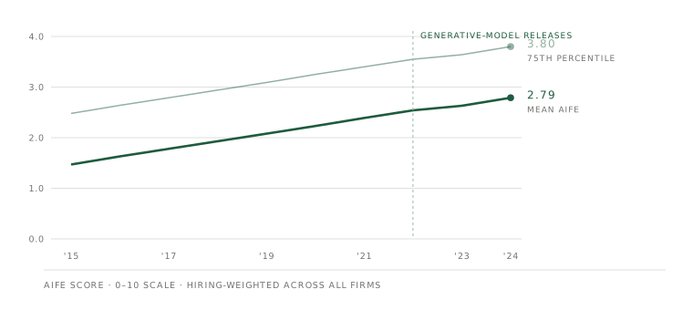
In the base year, mean AIFE was 1.47, reflecting a labor market where AI skills were present but peripheral. By 2024 it had nearly doubled to 2.79, a compound annual growth rate of 7.3%. The 75th percentile — which serves as our treatment threshold in §5 — rose from 2.48 to 3.80, indicating that leading firms are pulling away from the median. The acceleration around 2022–2023 coincides with the release of large-scale generative models.
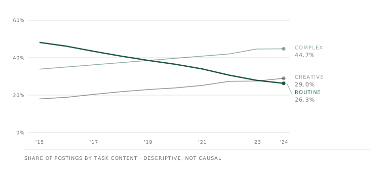
The share of routine postings fell from 48.2% in 2015 to 26.3% in 2024 — a decline of nearly 22 percentage points — mirrored by expansion of complex occupations from 33.9% to 44.7% and creative occupations from 18.0% to 29.0%. The magnitudes are consistent with AI substituting codifiable, rule-based tasks while complementing higher-order cognitive and creative work.
| Year | AIFE Mean | AIFE P75 | Routine % | Complex % | Creative % |
|---|---|---|---|---|---|
| 2015 | 1.47 | 2.48 | 48.17 | 33.87 | 17.96 |
| 2016 | 1.63 | 2.64 | 46.12 | 35.03 | 18.85 |
| 2017 | 1.78 | 2.79 | 43.39 | 36.20 | 20.41 |
| 2018 | 1.93 | 2.94 | 40.83 | 37.36 | 21.81 |
| 2019 | 2.08 | 3.09 | 38.53 | 38.52 | 22.96 |
| 2020 | 2.23 | 3.25 | 36.48 | 39.68 | 23.85 |
| 2021 | 2.39 | 3.40 | 33.98 | 40.84 | 25.18 |
| 2022 | 2.54 | 3.55 | 30.63 | 42.00 | 27.37 |
| 2023 | 2.63 | 3.64 | 27.88 | 44.62 | 27.50 |
| 2024 | 2.79 | 3.80 | 26.29 | 44.74 | 28.97 |
Hiring-weighted averages across all firms. P75 is the threshold used to define high-adoption firms in §5.
Two further properties are worth noting. Firm-level AIFE exhibits substantial cross-sectional dispersion: the interquartile range widens from 1.86 in 2015 to 2.42 in 2024, indicating that firms are diverging rather than converging. And trajectories exhibit strong temporal persistence: first-order autocorrelation is 0.94, and firms in the top quartile in year t have a 78% probability of remaining there at t+2. Together these suggest that AIFE trajectories may be predictable from current signals — a hypothesis we formalize in §6.
5Causal Analysis
The descriptive evidence documents two trends moving in opposite directions. We now ask whether they represent a causal effect of AI adoption or merely reflect confounded secular trends.
5.1 · Sample construction
The full panel contains approximately 3.1 million firm–year observations. We impose three restrictions: panel continuity — each firm must appear in at least three consecutive years, which drops 38.2% of observations, predominantly small firms with intermittent posting activity; minimum posting count — at least five postings per year, so the firm-level score aggregates over a minimally informative set; and non-missing controls. The resulting estimation sample contains 223,659 firm–year observations from 41,247 unique firms across 72 countries and 18 two-digit NAICS sectors. It over-represents larger, more established firms relative to the full population.
A note on generated regressors. Our main independent variable is itself the output of a machine-learning pipeline, and standard OLS and 2SLS standard errors do not account for estimation error in a generated regressor. We therefore report two sets throughout: analytic standard errors clustered at the firm level, treating AIFE as observed, and pipeline-bootstrap standard errors that resample the entire measurement pipeline — from teacher labeling through student inference to regression — over 500 iterations. In all specifications the bootstrap errors are within 15% of the analytic ones.
5.2 · Two-way fixed effects
where i, j(i) and t index firms, two-digit NAICS industries and years. The dependent variable is the firm's share of new postings classified as routine, complex or creative. The main independent variable is one-year lagged AIFE; this lag structure captures delayed workforce adjustment and mitigates simultaneity bias. Controls comprise log total postings as a scale proxy, log firm age, and the lagged dependent variable.1 The terms μi and δj(i),t are firm and industry-by-year fixed effects, the latter absorbing industry-wide trends so that β is identified from within-industry, within-firm variation.
| Routine (1) | Routine (2) | Creative (3) | Creative (4) | |
|---|---|---|---|---|
| AIFEi,t−1 | −0.024*** | −0.021*** | 0.022*** | 0.018*** |
| Log(total postings) | −0.006* | −0.005** | 0.009*** | 0.008*** |
| Log(firm age) | −0.012** | −0.009* | 0.005 | 0.003 |
| Industry × Year FE | No | Yes | No | Yes |
| Observations | 223,659 | 223,659 | 223,659 | 223,659 |
| Within R² | 0.142 | 0.187 | 0.115 | 0.153 |
Firm FE included throughout. *** p < 0.01; ** p < 0.05; * p < 0.10. Standard errors clustered at the firm level.
In the preferred specification the coefficient on lagged AI intensity is −0.021 for the routine share and +0.018 for the creative share. Economically, a one-unit increase in a firm's AIFE score is associated with a 2.1 percentage-point decline in routine hiring and a 1.8 point increase in creative hiring in the subsequent year. The coefficient on firm size is negative for routine and positive for creative, suggesting larger firms are already structurally shifting toward non-routine work; controlling for this scale gradient ensures the AI coefficient does not conflate intensity with a generic large-firm effect.
1 Including the lagged dependent variable in a short-panel fixed-effects model introduces Nickell bias of order O(1/T). With T = 9 the bias is approximately −12.5%. We verify that dropping the lagged dependent variable leaves the coefficient of interest essentially unchanged (Appendix N).
5.3 · Dynamic effects and parallel trends
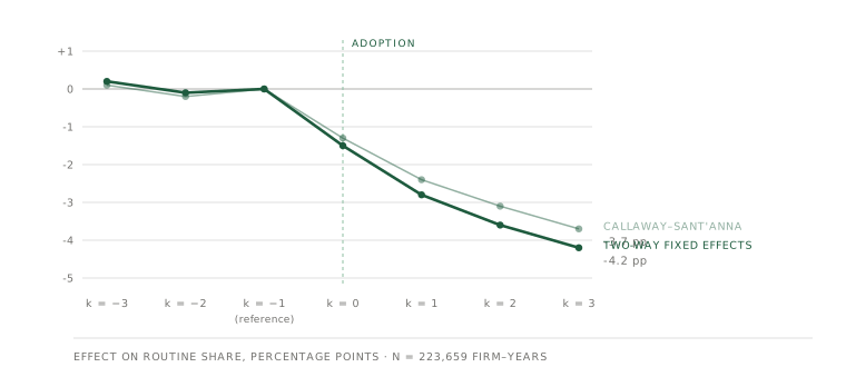
The TWFE model assumes a linear and constant effect and does not allow verification of parallel trends. We therefore classify a firm as an adopter in the first year its AIFE score exceeds the 75th percentile of the cross-sectional distribution, and estimate an event study with k = −1 omitted as reference.
Addressing staggered-adoption bias. Because firms adopt at different times, the classic TWFE event-study estimator can produce biased estimates when treatment effects are heterogeneous across cohorts or over time. In our setting the estimated effects grow monotonically from k = 0 to k = 3 — precisely the pattern susceptible to contamination. We therefore report a second set of estimates using the Callaway and Sant'Anna (2021) estimator, which constructs group-time average treatment effects free of forbidden comparisons between early and late adopters, using the not-yet-treated as the comparison group.
| Event time | TWFE | SE | CS (2021) | SE |
|---|---|---|---|---|
| Pre-treatment | ||||
| k = −3 | 0.002 | (0.004) | 0.001 | (0.005) |
| k = −2 | −0.001 | (0.003) | −0.002 | (0.004) |
| k = −1 | Omitted reference period | |||
| Post-treatment | ||||
| k = 0 | −0.015*** | (0.004) | −0.013*** | (0.005) |
| k = 1 | −0.028*** | (0.005) | −0.024*** | (0.006) |
| k = 2 | −0.036*** | (0.006) | −0.031*** | (0.008) |
| k = 3 | −0.042*** | (0.007) | −0.037*** | (0.009) |
Three findings emerge. First, the results satisfy parallel trends: pre-treatment coefficients are small and statistically indistinguishable from zero under both estimators, confirming that prior to becoming high-intensity adopters these firms were not already shedding routine jobs at a differential rate. Second, a clear structural break occurs at adoption, and the coefficient continues to decline to −0.042 by k = 3, suggesting that displacement effects are not transient shocks but trigger a persistent reorganization of the firm's production function. Third, the Callaway–Sant'Anna estimator yields qualitatively identical results, attenuated by 10–15% with wider confidence intervals — indicating that heterogeneity bias is present but quantitatively modest.
5.4 · Instrumental variable: shift-share design
Despite extensive controls, a residual endogeneity concern remains: an unobserved factor such as the appointment of a technology-oriented CEO could simultaneously drive AI adoption and workforce restructuring. We construct a shift-share instrument that leverages historical occupational structure:
where the shares are firm i's employment proportions in occupation o during the pre-sample period 2012–2015, and the shifts are national-level growth rates of mean AIFE in occupation o at time t, computed leave-one-out to exclude firm i's own postings and avoid mechanical correlation. Firms that historically specialized in tasks that later experienced rapid AI development are exposed to the technological shock for reasons unrelated to their current strategic choices.
Identifying assumptions. Under the exogenous-shares interpretation, identification requires that firms' pre-period occupational shares are uncorrelated with unobserved determinants of subsequent hiring composition, conditional on controls — plausible if occupational structure in 2012–2015 was determined by historical industry specialization rather than anticipation of the post-2015 AI wave. Under the exogenous-shifts interpretation, identification requires that national growth rates are exogenous, in the sense that no single firm drives the national trend in any occupation; the leave-one-out construction and the large number of occupations (468 SOC codes) support this.
| Share Routine | Share Creative | |
|---|---|---|
| Panel A · First stage (dep. var.: AIFEit) | ||
| Bartik IV (Zit) | 0.842*** (0.017) | |
| Kleibergen–Paap F | 2,340.5 | |
| Panel B · Second stage | ||
| AIFEit (instrumented) | −0.038*** | 0.029*** |
| Log(total postings) | −0.004* | 0.007*** |
| Log(firm age) | −0.008 | 0.002 |
| Observations | 223,659 | 223,659 |
We acknowledge that the very high first-stage F-statistic warrants scrutiny. Given that both the shares and the shifts are ultimately derived from job-posting data, a near-mechanical link is conceivable. The share–shift interaction operates through distinct channels — the shares are fixed at pre-period values while the shifts capture national leave-one-out trends over 2016–2024 — and we verify robustness to dropping the largest 10% of firms, which could dominate national trends. The IV estimates are nearly twice the OLS magnitudes, consistent with attenuation from measurement error in the generated regressor.
5.5 · Heterogeneity
| HICs | LMICs | Large | SMEs | |
|---|---|---|---|---|
| AIFEi,t−1 | −0.026*** | −0.013** | −0.029*** | −0.008* |
| Equality test (p) | 0.042 | 0.001 | ||
| Observations | 134,195 | 89,464 | 111,829 | 111,830 |
| Within R² | 0.195 | 0.132 | 0.210 | 0.104 |
The results reveal a pronounced automation divide. The substitution effect is nearly twice as large in high-income countries as in low- and middle-income ones, consistent with the factor-price channel: in high-wage, capital-deep environments the incentive to substitute routine labor with AI is significantly stronger, while in developing regions where labor is cheaper the pressure to automate is attenuated. Firm-scale heterogeneity is similarly stark — the coefficient for large firms is −0.029, whereas for SMEs the effect is small and only marginally significant, indicating that AI-driven workforce restructuring requires a scale of operation and capital investment currently concentrated among market leaders.
5.6 · Robustness
1. Treatment threshold sensitivity. Re-estimating the event study across adoption thresholds from the 30th to the 95th percentile, the effect scales monotonically from −0.007 to −0.048. This dose-response relationship — deeper AI integration leading to sharper declines in routine hiring — strengthens the causal interpretation by ruling out threshold artifacts.
2. Sector composition. Excluding all firms in NAICS 51 attenuates the coefficient only slightly, from −0.021 to −0.018, confirming that AI acts as a general-purpose technology rather than an IT-sector phenomenon. Manufacturing-only estimates yield −0.025, suggesting goods-producing sectors experience at least as strong a displacement effect.
3. Inference. Clustering at the two-digit NAICS level increases the standard error from 0.004 to 0.007 but preserves significance; two-way clustering by firm and year produces similar results.
4. Alternative controls. Replacing log total postings with log revenue yields a virtually identical coefficient of −0.020. Adding country-by-year fixed effects attenuates the estimate modestly to −0.018, consistent with some adoption being driven by country-level diffusion rather than firm-level choices.
5. Measurement robustness. Re-estimating on the subsample of firms whose AIFE score rests on at least 20 postings per year strengthens the coefficient to −0.025, consistent with classical attenuation bias in the baseline and directionally aligned with the OLS-to-IV amplification in §5.4.
5.7 · Summary and implications for prediction
The causal analysis establishes three regularities: a one-unit AIFE increase causes a 2.1 pp decline in routine hiring, or 3.8 pp under IV; the effect deepens monotonically over three post-adoption years; and the magnitude varies systematically across income levels and firm sizes. These are structural parameters — they characterize how the labor market responds to adoption, conditional on adoption occurring. They do not address which firms will experience AIFE increases, and when. If trajectories are themselves predictable, the causal effect sizes become directly actionable.
6Predictive Early Warning System
6.1 · Problem formulation
For firm i at time t we predict AIFEi,t+h at horizons h ∈ {1, 2, 3} years. We predict AIFE rather than employment outcomes directly for a structural reason: AIFE is the upstream causal variable whose downstream effects are identified in §5, so predicting it and applying the causal estimate yields forecasts interpretable through a known structural relationship rather than a black-box association.
6.2 · Semantic Leading Indicators
The scalar AIFE score is a lossy compression of the semantic information in job postings. Consider a manufacturing firm whose postings mention machine learning for the first time, but only in optional qualifications for one role. Its score changes marginally — yet in embedding space the firm's representation has shifted toward the AI cluster centroid, a leading indicator of adoption that precedes the scalar increase.
Let ēit be the mean [CLS] embedding across firm i's postings in year t, and μ*st the mean embedding of frontier postings (AIFE ≥ 8) in the same sector and year. We define three features:
- Semantic velocity — the change in cosine similarity between the firm centroid and the frontier, measuring how fast the firm's hiring language is converging on frontier vocabulary. Positive values indicate the firm is moving toward the frontier faster than the frontier itself is evolving.
- Semantic dispersion — the within-firm variance of posting embeddings. Firms in transition should exhibit elevated dispersion, with some roles reflecting legacy operations while others embody the post-adoption equilibrium; the inverted-U pattern serves as a leading indicator of imminent acceleration.
- Frontier distance — the Mahalanobis distance from the firm centroid to the sector frontier, computed in the top-64 principal component subspace. This captures room to grow: firms far from the frontier have more adoption headroom.
Extraction requires no additional forward passes; embeddings come from the same run that produces the scores, adding under 8% overhead. Granger-causality tests confirm all three provide statistically significant incremental predictive power beyond the autoregressive component, with semantic velocity strongest (ΔR² = 0.034).
6.3 · Forecasting architecture
We adopt the Temporal Fusion Transformer, which offers three properties well suited to a panel setting: variable selection networks that softly select the most informative features at each step, critical because the relative importance of lagged AIFE against the semantic indicators shifts with horizon; temporal self-attention whose weights are directly inspectable; and static covariate encoders that condition temporal dynamics on time-invariant features such as country and sector.
Causal-consistency regularizer. A novel feature of the architecture penalizes predictions inconsistent with the causal structure estimated in §5. A model that forecasts AIFE changes implying displacement outside the empirically estimated dose-response envelope is producing structurally implausible forecasts. We operationalize this as a hinge loss that imposes zero penalty inside the plausible range and a quadratic penalty on structurally implausible extremes:
The regularizer creates a direct architectural link between the causal-inference contribution and the prediction model, acting as an inductive bias that embeds the paper's own empirical findings into the loss function.
6.4 · Uncertainty quantification
Point forecasts, however accurate, are insufficient for policy use; decision-makers require calibrated prediction intervals. Parametric intervals are fragile under distributional misspecification, and quantile-regression intervals lack finite-sample coverage guarantees. We therefore adopt split conformal prediction, which provides distribution-free marginal coverage under minimal assumptions.
Standard exchangeability fails here, because observations within a firm are serially correlated and the data-generating process shifts over time. We therefore use a weighted conformal framework that assigns importance weights decaying exponentially in the distance between calibration and test years, providing approximate coverage under covariate shift. In practice, with a one-year half-life and four to six calibration years, the correction term is below 0.02 at all horizons.
6.5 · Evaluation
We employ an expanding-window design with strict temporal separation across four windows, training on 2015 onward, validating on the following year, reserving the next for conformal calibration only, and testing on the last. The calibration year is never used for gradient updates.
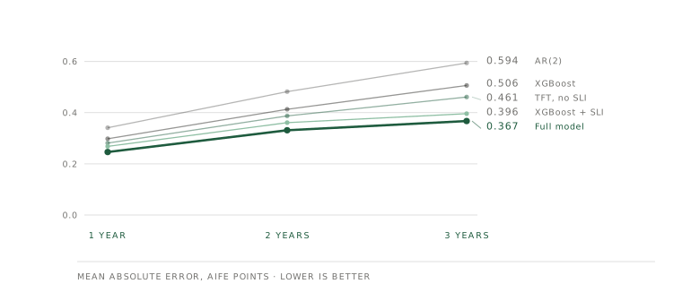
| Model | h=1 MAE | h=1 R² | h=2 MAE | h=2 R² | h=3 MAE | h=3 R² |
|---|---|---|---|---|---|---|
| AR(2) | .341 | .791 | .482 | .596 | .594 | .413 |
| XGBoost | .298 | .839 | .413 | .700 | .506 | .568 |
| TFT (no SLI) | .281 | .857 | .387 | .736 | .461 | .637 |
| XGBoost + SLI | .268 | .869 | .361 | .767 | .396 | .728 |
| Full model | .246 | .889 | .331 | .802 | .367 | .763 |
Three patterns emerge. The full model dominates at all horizons, with MAE reductions of 18–31% relative to AR(2) and 8–14% relative to XGBoost without the semantic indicators. The indicators provide the largest marginal gain at longer horizons: at h = 1 the improvement is modest, because the autoregressive component carries most of the signal, but at h = 3 the gain is substantial. And the TFT architecture outperforms XGBoost on the same feature set, with the gap widening at longer horizons, because temporal self-attention identifies relevant historical patterns that tree-based models processing each time step independently cannot exploit.
Coverage. The TFT's native quantile intervals undercover at all horizons, with the shortfall growing from 2.7 percentage points at h = 1 to 7.3 at h = 3 — a known failure mode of quantile regression under distribution shift. Conformal intervals achieve or exceed nominal coverage at every horizon and level, with overcoverage bounded by 1.1 points, and with comparable or narrower widths.
Feature importance. At h = 1, autoregressive lags dominate with combined weight 0.42 while the semantic indicators contribute 0.32. By h = 3 the profile inverts: the indicators account for 46% of model attention while lagged AIFE falls to 25%. Semantic velocity is consistently the most important, consistent with the Granger-causality ordering.
6.6 · From forecasts to displacement early warnings
The practical payoff is the conversion of AIFE forecasts into labor-market early warnings via the causal link. Because the mapping is linear, the coverage guarantee on AIFE forecasts propagates directly to the displacement interval.
Limitations of the early warning system. The displacement forecasts inherit two sources of uncertainty: AIFE prediction error, quantified by the conformal interval, and causal parameter uncertainty, quantified by the standard error of β̂IV. The intervals above capture only the first. A fully Bayesian treatment would propagate both; causal parameter uncertainty adds approximately ±0.8 percentage points at the median predicted change, a modest contribution relative to prediction uncertainty.
7Conclusion
This paper has developed a three-part system for understanding and anticipating AI-driven labor-market disruption: a measurement pipeline that quantifies firm-level AI adoption at scale, a causal analysis that identifies the structural consequences of adoption, and a predictive system that combines forecasts with causal estimates to produce actionable displacement warnings.
Measurement. The pipeline demonstrates that the reasoning capabilities of a frontier LLM can be transferred to a lightweight encoder at a cost reduction of 370×, while preserving 93% correlation with human expert labels. It outperforms all tested baselines. The approach is generalizable: the same teacher–student–human architecture could measure other latent economic constructs from unstructured text.
Causal validation. Firms that increase AI intensity reduce routine hiring by 2.1 pp per unit of AIFE and increase creative hiring by 1.8 pp. The effect deepens monotonically over three post-adoption years, consistent with permanent task reorganization. Instrumenting for endogeneity amplifies the estimates, confirming attenuation bias in OLS. The displacement is twice as large in high-income countries and concentrated among large firms — an automation divide with significant policy implications.
Predictive early warning. By extracting semantic leading indicators from the pipeline's intermediate representations and embedding them in a Temporal Fusion Transformer with causal-consistency regularization, the system forecasts trajectories at one-to-three-year horizons with error reductions of 18–31% over autoregressive baselines, with distribution-free coverage guarantees.
The integrated system. Each contribution depends on the preceding one. Prediction requires a validated measure to define the target variable; displacement forecasts require credible causal estimates to translate predictions into consequences. Neither component alone produces actionable intelligence: measurement without prediction is retrospective, prediction without causal identification is uninterpretable, and causal estimates without prediction are not forward-looking.
Author contributions
Liqian Yan led the team, devised the theoretical model explaining why AI changes hiring, made the predictions about substitution and complementarity, ran the numerical simulations, and wrote the policy section. Yintong Chen developed the empirical strategy, including the dynamic event-study design and the shift-share instrumental variable. Zichun Qiu built the data engineering — organising over 400 million raw postings, training the ModernBERT student, and constructing the teacher–student pipeline. The work was supervised by Professors Mingmao Deng and Jingping Chen of the Shanghai University of International Business and Economics.
Limitations
Demand-side measurement only. The pipeline observes labor demand — job postings — but not labor supply: worker skills, educational attainment, career transitions. We therefore cannot measure skill mismatches, equilibrium wages, or welfare consequences.
Web-crawled corpus coverage. The WDC corpus over-represents English-language, digitally posted positions in formal-sector firms. Results may not generalize to informal labor markets, small firms with no online presence, or countries with low internet penetration.
Generated regressor. AIFE is a model-generated proxy for latent AI adoption intensity. It captures stated hiring intent, not verified deployment. External validation against independent measures — IT capital expenditure, patent filings, software licences — would strengthen the measurement claim.
Prediction horizon. The forecasting system performs well at one-to-three-year horizons but relies on the assumption that structural relationships between semantic features and trajectories remain stable. Discontinuous technological shifts could invalidate longer-horizon forecasts; the causal regularizer mitigates but does not eliminate this risk.
Uncertainty propagation. The displacement forecasts incorporate AIFE prediction uncertainty but treat the causal parameter as fixed.
Future Directions
Three extensions follow naturally. First, integrating supply-side data — worker skills and career trajectories — with the demand-side panel would enable a matching model that captures both sides of the reallocation process. Second, the staggered nature of AI adoption across countries creates opportunities for cross-national policy evaluation, estimating whether retraining subsidies, educational reforms or regulatory interventions moderate the displacement effects. Third, extending the pipeline to adjacent technological transitions such as robotics and green technology would test the generalizability of the knowledge-distillation approach. On the prediction side, integrating exogenous technology-shock indicators — foundation-model release dates, venture capital flows into AI startups — as known future inputs could improve long-horizon forecasts.
References
An abridged list; the complete bibliography and all appendices are in the PDF.
- Acemoglu, D., & Autor, D. (2011). Skills, tasks and technologies: Implications for employment and earnings. Handbook of Labor Economics, 4B, 1043–1171.
- Acemoglu, D., & Restrepo, P. (2018). The race between man and machine. American Economic Review, 108(6), 1488–1542.
- Acemoglu, D., & Restrepo, P. (2020). Robots and jobs: Evidence from US labor markets. Journal of Political Economy.
- Autor, D. H., & Dorn, D. (2013). The growth of low-skill service jobs and the polarization of the US labor market. American Economic Review, 103(5), 1553–1597.
- Autor, D. H., Levy, F., & Murnane, R. J. (2003). The skill content of recent technological change. Quarterly Journal of Economics, 118(4), 1279–1333.
- Bessen, J. E. (2019). AI and jobs: The role of demand. NBER Working Paper No. 24235.
- Borusyak, K., Hull, P., & Jaravel, X. (2022). Quasi-experimental shift-share research designs. Review of Economic Studies.
- Brynjolfsson, E., & McAfee, A. (2014). The Second Machine Age. W. W. Norton.
- Callaway, B., & Sant'Anna, P. H. C. (2021). Difference-in-differences with multiple time periods. Journal of Econometrics.
- Chen, T., & Guestrin, C. (2016). XGBoost: A scalable tree boosting system. KDD.
- Cortés, G. M., Jaimovich, N., Nekarda, C. J., & Siu, H. E. (2016). Reallocation across occupations and the decline of middle-skill employment. FEDS 2016-0001.
- De Chaisemartin, C., & D'Haultfœuille, X. (2020). Two-way fixed effects estimators with heterogeneous treatment effects. American Economic Review.
- Deming, D. J. (2017). The growing importance of social skills in the labor market. Quarterly Journal of Economics, 132(4), 1593–1640.
- Devlin, J., Chang, M.-W., Lee, K., & Toutanova, K. (2019). BERT: Pre-training of deep bidirectional transformers. NAACL-HLT.
- Efron, B., & Tibshirani, R. (1994). An Introduction to the Bootstrap. Chapman & Hall.
- Eloundou, T., Manning, S., Mishkin, P., & Rock, D. (2023). GPTs are GPTs: An early look at the labor market impact potential of large language models.
- Felten, E., Raj, M., & Seamans, R. (2021). Occupational, industry, and geographic exposure to artificial intelligence. Strategic Management Journal.
- Frey, C. B., & Osborne, M. A. (2017). The future of employment. Technological Forecasting and Social Change, 114, 254–280.
- Goldin, C., & Katz, L. F. (2008). The Race between Education and Technology. Harvard University Press.
- Goldsmith-Pinkham, P., Sorkin, I., & Swift, H. (2020). Bartik instruments: What, when, why, and how. American Economic Review.
- Goodman-Bacon, A. (2021). Difference-in-differences with variation in treatment timing. Journal of Econometrics.
- Goos, M., & Manning, A. (2007). Lousy and lovely jobs. American Economic Review, 97(2), 118–122.
- Graetz, G., & Michaels, G. (2018). Robots at work. Review of Economics and Statistics, 100(5), 753–768.
- Katz, L. F., & Murphy, K. M. (1992). Changes in relative wages, 1963–1987. Quarterly Journal of Economics, 107(1), 35–78.
- Loshchilov, I., & Hutter, F. (2019). Decoupled weight decay regularization. ICLR.
- Niculescu-Mizil, A., & Caruana, R. (2005). Predicting good probabilities with supervised learning. ICML.
- Noy, S., & Zhang, W. (2023). Experimental evidence on the productivity effects of generative artificial intelligence. Science.
- Pagan, A. (1984). Econometric issues in the analysis of regressions with generated regressors. International Economic Review.
- Sun, Y., & Abraham, S. (2021). Estimating dynamic treatment effects in event studies with heterogeneous treatment effects. Journal of Econometrics.
- Webb, M. (2020). The impact of artificial intelligence on the labor market. Working paper.
- Wei, J., et al. (2022). Emergent abilities of large language models. TMLR.
- Xu, X., et al. (2023). AI adoption and labor demand restructuring: Evidence from Chinese recruitment data.
- Zeng, Y., et al. (2025). Generative AI and income distribution under capital–skill complementarity.
- Zhang, Y., & Dan, W. (2025). Generative AI exposure and hiring demand: Evidence from Chinese recruitment data.